Quant Trading
A time series case study.
Background
For a securities exchange \(E\), participants of \(E\) include buyers and sellers, each submitting orders at various values of price \(P\) and volume \(V\) the buyers are willing to buy, and sellers willing to sell. The culmination of these orders create an orderbook, \(O(t)\), commonly referred to as level 2 (L2) market order data. At any given time \(t\), the “best bid, best offer” (BBO) is the best price \(P_{\text{BBO}}(t)\) at which someone is willing to buy and sell. Whenever a buy/sell order is submitted that the sell/buy orders can fulfill, the order is filled. \(P_{\text{BBO}}(t)\) is subject to the participants’ contributions to the buy/sell distribution of limit orders pending to be executed. If an order is traded using \(P_{\text{BBO}}\), this would be subject to ‘‘taker“ trading fees; if a limit order is submitted for \(P_{\text{BBO}}\pm \delta \) \(\left(\delta>0\right)\), the order is subject to ‘‘maker” trading fees. Usually, exchanges reduce maker fees (sometimes negative) to incentivize liquidity/volume for their exchange.
Objective
Is there a consistently profitable (algorithmic) methodology of submitting a series of buy/sell orders in exchange E=Bitmex, instrument=XBTUSD (Bitcoin)?
Computational, Analytical Framework
A generalizable algorithmic framework is as follows. A timing and sizing of wagers (denoted by \(f\left(\vec{p}_{\text{predict}}(t), \vec{p}_{\text{threshold}}(t),\vec{W}\left(\vec{p}_{\text{predict}}(t), \vec{p}_{\text{threshold}}(t), O(t)\right),O(t) \right)\) is applied on \(O(t)\), as time \(t\) monotically increases in observable increments of \(\Delta t(t)\). For \(t=t_{\text{current}}\in\left[T_{\text{backward}},t_{\text{current}}\right]\), \(\forall t\), a set of calculated predictor features, \(\vec{X}_{\text{training}}(t)\), and for \(t=t_{\text{current}}\in\left(t_{\text{current}},T_{\text{forward}}\right]\), historical signals of truth, \(y_{\text{training, truth}}(t)\), are assembled to construct an optimization problem: a model \(M\) and modeling parameters \(\vec{A}\) is proposed for cost (objective) function \(C = C\left(M\left(\vec{A}, \vec{X}_{\text{training}}(t)\right),y_{\text{training, truth}}(t)\right)\) to arrive at an optimal set of parameters, \(\vec{A}^{*}\):
\[ \begin{equation} \vec{A}^{*} = \underset{\vec{A}}{\text{argmin }} C\left(M\left(\vec{A},\vec{X}_{\text{training}}(t)\right),y_{\text{training, truth}}(t)\right)\label{eq:1}. \end{equation} \]
Thus, through validation, regularization, and generalization, ensure \(M\left(\vec{A}^{*},\vec{X}_{\text{test}}(t)\right) = \vec{p}_{\text{predict}}(t) > \vec{p}_{\text{threshold}}\) for signals of truth outside the training set, \(y_{\text{test, truth}}(t)\). We end up having to use numerical optimization techniques and high performance computing (C++ is used to handle hundreds of millions of rows of tick data) to solve such functions for parameters \(T_{\text{backward}}\), \(T_{\text{forward}}\), iterative hypothesizing of \(\vec{X}_{\text{training}}(t)\), \(\vec{p}_{\text{threshold}}(t)\), realistic throttling of \(\Delta t(t)\) to account for a production environment latency (\(\Delta t(t) = \hat{\Delta} t\)), and design of model \(M\).
Results
For out-of-sample \(\vec{X}_{\text{test}}(t)\) predictors and \(y_{\text{test, truth}}(t)\) signals of truth, a backtest is performed to evaluate performance emulating a replay of \(O(t)\), at first trading at \(P_{\text{BBO}}(t)\):
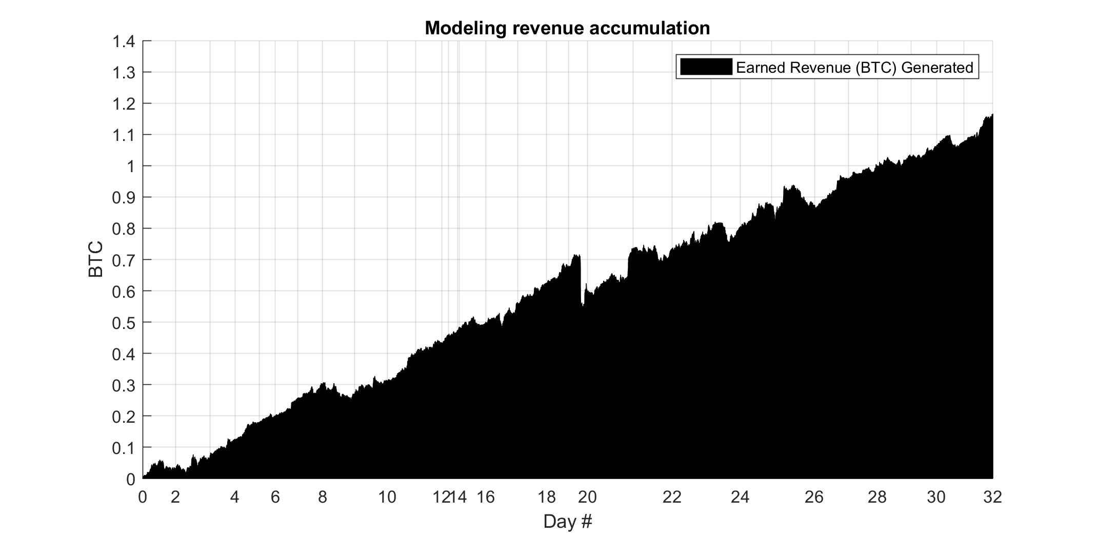 |
| Test date range: March 26, 2024 to April 25, 2024 (32 days); \(\approx 300M\) ticks; trading fee= a 0.00%; \(\displaystyle\sum_{i} W_{i} \approx 10,000\text{BTC}\) of wager volume made (at any given time, \(\le\) 1BTC of positions are placed), consisting of \(\frac{N_{\text{bets}}}{2}\approx 50000\) total full trades (1 full trade being 1 \(\left(\text{buy, sell}\right)\) combination of positions), each full trade having an associated total trading cost to execute. |
However, in a high frequency environment, this would be sensitive to ‘‘taker" trading fees for trading at \(P_{\text{BBO}}\). A trading fee analysis shows that a maker fee (versus a taker fee) would be advantagous; maker fees can commonly be anywhere from \(\left[-0.025, .025 \right] \% \). Backtesting the performance for trading fee of this range:
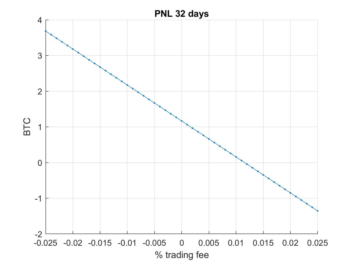 |
| PnL \(\ge 0\) for trading taker fee \(\le 0.011\%\) for trading at \(P_{\text{BBO}}(t)\); however, maker fees are usually lower. To be subject to maker fees, algorithmically orders would need to be ensured to be maker orders, even if the orders are for price \(P_{\text{BBO}}\pm 0.5\) through the exchange API. If by doing so reduces return, then a lower \(\left(< \right)\) trading fee will compensate for providing liquidity for the exchange \(E\) (as seen above). |
Conclusion
As a proof of concept, this framework seemed to be viable for \(E=\)Bitmex, instrument\(=\)XBTUSD (BTC). Additionally, there are many exchanges, and many instruments in markets, this can be experimented on.
References
DailyCoin. Crypto Exchange Fees Comparison 2024: Who Has the Lowest Trading Fees? (2024, April 27). https://dailycoin.com/crypto-exchange-fees-comparison/