Blackjack
 |
Me and Edward Thorp, 2017. Mr. Thorp played a critical role in Blackjack history to mathematically find ways for a player to overcome a casino's edge of Blackjack and play profitably such that the player would have an edge over the casino; he wrote the first book on counting cards in 1962, Beat the Dealer. Mr. Thorp has been using mathematical models to beat the stock market since the 1960's, and reported that his personal investments yielded an annualized 20 percent rate of return averaged over 30 years (Forbes, Preston, 2017), reportedly operating a $300 million fund at times (Kurson, 2003). |
Contents
History
First written references of a card game resembling that of Blackjack is written between 1601 and 1602 originating from Spain (Wikipedia, 2022); the first record of the game in France occurs in 1888, and in Britain in the late eighteenth century. The card game and rules made its first appearance in the USA in the early nineteenth century, and later developed into an American variant which was renamed “Blackjack” around 1899. (Depaulis, 2010)
In USA, initially legalized in Nevada, casinos have been growing in popularity after World War II, particularly in Las Vegas and Reno. In the late 20th century, casinos became more popular in Native American Indian tribal land, as their legal jurisdiction allows for them. More recently, tribes have even been building casinos on non-tribal land they own to expand casino popularity further. Casino game offerings (slots and table games) have grown in popularity proportional to this casino popularity growth. In contrast to other casino games, Blackjack requires the player's decisions to have a big influence on the expected returns of play. With optimal play, the Blackjack player can reduce the casino advtange to zero or even make the game favorable to the player. With enough skill, adhering to mathematics and probability, a player can (in the long run) systematically win.
The work of Baldwin et al. (1956) presented the first viable mathematical approach for analyzing Blackjak and an optimized playing technique, known as basic strategy (Baldwin et al., 1956). This basic strategy is the first step of minimizing the casino advantage against the player. Ed Thorp (1962-1966) took the approach further, realizing that the expected return for a given hand varied with the composition of the undealt cards of the shoe. Thorp proposed a card counting method that would help identify instances when the odds were in the advantage of the player on a particular round. Thorp concluded that the player increasing his bet during these advantagaous times, could achieve a positive overall edge. Card counting developments continued after Thorp's work (Snyder, 2006).
In 1999, Petter Griffin went beyond Thorp and others to have a quantitative approach for analyzing other aspects of Blackjack strategy, including introducing the idea of multi-parameter counting systems, beyond that of the single-parameter counting system Ed Thorp first proposed (Griffin, 1999). To this day, methods are being innovated to continue to beat Blackjack and other table games, despite the countermeasures by the casinos. In 2008, Don Johnson won $15 million at Blackjack, betting $100,000 a hand, and James Grosjean has written extensive work on methods beyond that of counting.
Rules
Blackjack is a card game offered in casinos throughout the world. Rules vary depending on jurisdiction and consent of casino, but the overarching rules are the same: the goal of a player is beating a dealer by either:1) player drawing a hand value that is higher than the dealer's hand value, or
2) the dealer drawing a hand value that goes over 21 and the player's does not, or
3) player drawing a hand value of 21 on first two cards, when the dealer does not.
A player makes decisions on hands to achieve the above goals; Hit (H), Stand/Stay (S), Surrender (SR), Double (D), Split (SP). Depending on the hand composition of the player, certain actions are permitted.
Objective
Is there a way to consistently overcome the house edge, such that this game becomes profitable for the player? This study shows there is, and there is a lot of opportunity to do so.Analytical Framework: Objective Function Formulation (Maximizing Return, \(E\left[R\left(d,\pi\left(\vec{\alpha}\right),\vec{l}\right)\right]\))
There are 10 unique values of cards in the game of Blackjack, seen below. The number of 52 card decks in a shoe is \(D\). For \(D\) decks, for \(M\) drawn cards and \(\tilde{M}\) undealt cards, the number of cards in a shoe is \(M+\tilde{M} = 52D\). The number of drawn cards for a card type \(j\) is \(m_{j}\) and the number of undealt cards of type \(j\) is \(\tilde{m}_{j}\), such that \(m_{j} + \tilde{m}_{j} = \nu_{j}\). For \(52D\) total cards in a shoe, there are \(\tilde{\nu}_{j}\) cards of card type \(j\) in the shoe, where \(\nu_{j} = 52Dl_{j}^{0},\) \(l_{j}^{0}\) defined below. We'll define the depth of the shoe \(d = \frac{M}{52D}\) and \(\tilde{d} = \frac{\tilde{M}}{52D} = 1 - d\).| Card type \(j\) | Card | Value | # of cards in shoe, \(\nu_{j}\) | likelihood \(\left(l_{j}^{0}\right)\) at depth \(d=0\), \(M=0\) (zero depth) |
| 1 | A | 1 or 11 | 4D | 4/52 = 1/13 |
| 2 | 2 | 2 | 4D | 4/52 = 1/13 |
| 3 | 3 | 3 | 4D | 4/52 = 1/13 |
| 4 | 4 | 4 | 4D | 4/52 = 1/13 |
| 5 | 5 | 5 | 4D | 4/52 = 1/13 |
| 6 | 6 | 6 | 4D | 4/52 = 1/13 |
| 7 | 7 | 7 | 4D | 4/52 = 1/13 |
| 8 | 8 | 8 | 4D | 4/52 = 1/13 |
| 9 | 9 | 9 | 4D | 4/52 = 1/13 |
| 10 | 10, J, Q, K | 10 | 16D | 16/52 = 4/13 |
When dealing, we sample \(M\) total cards without replacement, and the likeliness to draw a card of type \(j\), \(l_{j}\), is subject to change. What is the probability we have exactly \(m_{j}\) \((j = 1,…,10)\) cards in our sample of \(M=\sum_{j} m_{j}\) dealt cards? All the possible ways (combinations) we can choose our sample of \(m_{j}\) \((j = 1,…,10)\) occur with the same probability. How many different such ways are there? There are \({{\nu_{j}}\choose{m_{j}}}=\frac{\nu_{j}!}{m_{j}!(\nu_{j} - mu_{j})!}\) ways for each \(j\), and across all \(j\), \(\prod_{j} {{\nu_{j}}\choose{m_{j}}}\) . The total number of \(M\) subsets of \(52D\) gives the size of the total sample space, \({{52D}\choose{M}}=\frac{(52D)!}{M!(52D - M)!}\). So, the probability we have exactly \(m_{j}\) \((j = 1,…,10)\) cards in our sample of \(M=\sum_{j} m_{j}\) dealt cards is
\[ \begin{align} P\left(\vec{m}, \vec{\nu}, 52D, M\right) = \frac{\prod_{j} {{\nu_{j}}\choose{m_{j}}}}{{{52D}\choose{M}}} = \frac{M!(52D - M)!}{\left(52D\right)!}\prod_{j} \frac{v_{j}!}{m_{j}!\left(v_{j} - m_{j}\right)!}\label{eq:1} \end{align} \]
where
\[ \begin{align} \vec{m} = \newcommand\mycolv[1]{\begin{bmatrix}#1\end{bmatrix}} \mycolv{m_{1}\\.\\.\\.\\m_{10}}.\label{eq:2} \end{align} \]
Because \(M+\tilde{M} = 52D\) and \(m_{j} + \tilde{m}_{j} = \nu_{j}\), due to symmetry,
\[ \begin{align} P\left(\vec{m}, \vec{\nu}, 52D, M\right) = P\left(\vec{\tilde{m}}, \vec{\nu}, 52D, \tilde{M}\right)\label{eq:3} \end{align} \]
\[ \begin{align} P\left(\vec{\tilde{m}}, \vec{\nu}, 52D, \tilde{M}\right) = \frac{\prod_{j} {{\nu_{j}}\choose{\tilde{m}_{j}}}}{{{52D}\choose{\tilde{M}}}} = \frac{\tilde{M}!(52D - \tilde{M})!}{\left(52D\right)!}\prod_{j} \frac{v_{j}!}{\tilde{m}_{j}!\left(v_{j} - \tilde{m}_{j}\right)!}\label{eq:4} \end{align} \]
where
\[ \begin{align} \vec{\tilde{m}} = \newcommand\mycolv[1]{\begin{bmatrix}#1\end{bmatrix}} \mycolv{\tilde{m}_{1}\\.\\.\\.\\\tilde{m}_{10}}.\label{eq:5} \end{align} \]
This probability distribution for \(\tilde{m}_{j}\) in \(\eqref{eq:4}\) is a hypergeometric distribution. As (Werthamer, 2009) states, where \(\tilde{m} = \tilde{M}\vec{l}\), the distribution of \(\vec{l}\) can be found from \(\eqref{eq:4}\) \(\left(P\left(\tilde{M}\vec{l}, \vec{\nu}, 52D, \tilde{M}\right)\right)\) and in the asymptotic limit, the otherwise discrete variable \(\vec{l}\) becomes quasi-continuous, where \(\nu_{j} \gg 1\) for each \(j\), and \(\vec{l}\) can be closely approximated as a continuous variable, and will later be shown to be good approximations for small number of decks \(D\). The likelihood of drawing card value \(j\) as the next card is \(l_{j} = \frac{\tilde{m}_{j}}{\tilde{M}}\), where
\[ \begin{align} \vec{l} = \newcommand\mycolv[1]{\begin{bmatrix}#1\end{bmatrix}} \mycolv{l_{1}\\.\\.\\.\\l_{10}}.\label{eq:6} \end{align} \]
Using Stirling's approximation of \(n! \approx \sqrt{2\pi n}\left(\frac{n}{e}\right)^{n}\) on \(\eqref{eq:4}\), replacing \(\vec{\tilde{m}}\) with \(\tilde{M}\vec{l}\), we arrive at a continuous probability distribution function for \(\vec{l}\), the likelihood vector \(\eqref{eq:6}\):
\[ \begin{align} P\left(\tilde{M}\vec{l}, \vec{\nu}, 52D, \tilde{M}\right) \approx \underbrace{\frac{\sqrt{2\pi \tilde{M}}\left(\frac{\tilde{M}}{e}\right)^{\tilde{M}} \sqrt{2\pi (52D-\tilde{M})}\left(\frac{(52D-\tilde{M})}{e}\right)^{(52D-\tilde{M})}}{\sqrt{2\pi (52D)}\left(\frac{(52D)}{e}\right)^{(52D)}} }_\textrm{term 1} \prod_{j} \underbrace{ \left(\frac{\sqrt{2\pi \nu_{j}}\left(\frac{\nu_{j}}{e}\right)^{\nu_{j}}}{\sqrt{2\pi (\nu_{j} - \tilde{M}l_{j})}\left(\frac{\nu_{j}-\tilde{M}l_{j}}{e}\right)^{\nu_{j} - \tilde{M}l_{j}}\sqrt{2\pi \tilde{M}l_{j}}\left(\frac{\tilde{M}l_{j}}{e}\right)^{\tilde{M}l_{j}}}\right) }_\textrm{term 2} \label{eq:7} \end{align} \]
Term 1 in \(\eqref{eq:7}\) reduces to
\[ \begin{align} \frac{\sqrt{2\pi M}\sqrt{\tilde{M}}}{\sqrt{52D}}e^{-\tilde{M}}e^{(52D)}e^{-M}\tilde{M}^{\tilde{M}}\frac{M^{M}}{(52D)^{(52D)}} = \frac{\sqrt{2\pi M \tilde{M}}}{\sqrt{52D}} \frac{M^{M} \tilde{M}^{\tilde{M}} }{(52D)^{M} (52D)^{\tilde{M}}} = \sqrt{2\pi(52D) d \tilde{d}}d^{M} \tilde{d}^{\tilde{M}}, \label{eq:8} \end{align} \]
Term 2 in \(\eqref{eq:7}\) reduces to
\[ \begin{align} \frac{\sqrt{2\pi\nu_{j}}\left(\frac{\nu_{j}}{e}\right)^{\nu_{j}}}{\sqrt{2\pi(\nu_{j} - \tilde{M}l_{j})}\sqrt{2\pi\tilde{M}l_{j}}\left(\frac{\nu_{j}-\tilde{M}l_{j}}{e}\right)^{\nu_{j} - \tilde{M}l_{j}}\left(\frac{\tilde{M}l_{j}}{e}\right)^{\tilde{M}l_{j}}} = \underbrace{ \frac{\sqrt{\nu_{j}}}{\sqrt{2\pi(\nu_{j} - \tilde{M}l_{j})(\tilde{M}l_{j})}} }_\textrm{term 3} \underbrace{ \frac{\nu_{j}^{\nu_{j}}}{(\nu_{j} - \tilde{M}l_{j})^{\nu_{j} - \tilde{M}l_{j}}(\tilde{M}l_{j})^{\tilde{M}l_{j}}} }_\textrm{term 4}\label{eq:9} \end{align} \]
We set \(l_{j} = l_{j}^{0}(1 + \varepsilon_{j})\), as the likelihood of a card type \(j\) slightly deviates around \(l_{j}^{0}\) as depth \(d=\frac{M}{52D}\) varies. Term 3 from \(\eqref{eq:9}\) reduces to
\[ \begin{align} \frac{1}{\sqrt{2\pi}}\frac{\sqrt{52D}\sqrt{l_{j}^{0}}}{\sqrt{52Dl_{j}^{0} - l_{j}^{0}(1+\varepsilon_{j})\tilde{M}}\sqrt{l_{j}^{0}(1+\varepsilon_{j})\tilde{M}}} &= \frac{1}{\sqrt{2\pi}}\frac{\sqrt{52D}}{\sqrt{52Dl_{j}^{0} (1+\varepsilon_{j})\tilde{M} - l_{j}^{0}(1+\varepsilon_{j})^{2}\tilde{M}^{2}}} \\ & = \frac{1}{\sqrt{2\pi}}\frac{1}{\sqrt{52Dl_{j}^{0}}\sqrt{(1-\tilde{d})\tilde{d} + \varepsilon_{j}\tilde{d} - 2\varepsilon_{j}\tilde{d}^{2} - \varepsilon_{j}^{2}\tilde{d}_{j}^{2}}} \\ & = \frac{1}{\sqrt{2\pi\nu_{j}}}\frac{1}{\sqrt{d\tilde{d} + \varepsilon_{j}d\tilde{d} - \epsilon\tilde{d}^{2} - \tilde{d}^{2}\varepsilon_{j}}} \\ & = \frac{1}{\sqrt{2\pi\nu_{j}}}\frac{1}{\sqrt{(\tilde{d}+\tilde{d}\varepsilon_{j})(d - \tilde{d}\varepsilon_{j})}}\label{eq:11} \end{align} \]
Term 4 from \(\eqref{eq:9}\) reduces to
\[ \begin{align} \frac{(52Dl_{j}^{0})^{52Dl_{j}^{0}}}{(52Dl_{j}^{0} - l_{j}^{0}(1+\varepsilon_{j})(52D)\tilde{d})^{52Dl_{j}^{0}}(52Dl_{j}^{0} - l_{j}^{0}(1+\varepsilon_{j})(52D)\tilde{d})^{-l_{j}^{0}(1+\varepsilon_{j})(52D)\tilde{d}}(l_{j}^{0}(1+\varepsilon_{j})(52D)\tilde{d})^{l_{j}^{0}(1+\varepsilon_{j})(52D)\tilde{d}}} \label{eq:12} \end{align} \]
\[ \begin{align} &= \frac{(52Dl_{j}^{0} - l_{j}^{0}(1+\varepsilon_{j})(52D)\tilde{d})^{l_{j}^{0}(1+\varepsilon_{j})(52D)\tilde{M}}}{(1-(1+\varepsilon_{j})\tilde{d})^{52Dl_{j}^{0}}(l_{j}^{0}(1+\varepsilon_{j})(52D)\tilde{d})^{l_{j}^{0}(1+\varepsilon_{j})(52D)\tilde{d}}} \\ &=\frac{(1 - (1+\varepsilon_{j})\tilde{d})^{l_{j}^{0}(1+\varepsilon_{j})(52D)\tilde{d} - 52Dl_{j}^{0}}}{((1+\varepsilon_{j})\tilde{d})^{l_{j}^{0}(1+\varepsilon_{j})(52D)\tilde{d}}} \\ &= \frac{(1 - (1+\varepsilon_{j})\tilde{d})^{\nu_{j}\tilde{d}(1+\varepsilon_{j}) - \nu_{j}}}{((1+\varepsilon_{j})\tilde{d})^{\nu_{j}(1+\varepsilon_{j})\tilde{d}}} \\ &= e^{\nu_{j} \phi_{1}(\varepsilon_{j})}\label{eq:13} \end{align} \]
where \(\phi_{1}(\varepsilon_{j})\) in \(\eqref{eq:13}\) is
\[ \begin{align} \phi_{1}(\varepsilon_{j}) &= \varepsilon_{j}\tilde{d}ln\left(1 - (1+\varepsilon_{j})\tilde{d}\right) - (1 + \varepsilon_{j})\tilde{d}ln((1+\varepsilon_{j})\tilde{d}) + \tilde{d}ln(1 - (1+\varepsilon_{j})\tilde{d}) - ln(1 - (1+\varepsilon_{j})\tilde{d}) \\ &= (\varepsilon_{j}\tilde{d} + \tilde{d} - 1)ln(f-\varepsilon_{j}\tilde{d}) - (1+\varepsilon_{j})\tilde{d}ln(\tilde{f} + \varepsilon_{j}\tilde{d}) \\ &= ln\left(\frac{(d - \varepsilon_{j}\tilde{d})^{\varepsilon_{j}\tilde{d} + d - 1}}{(\tilde{h} + \varepsilon_{j}\tilde{h})^{(1+\varepsilon_{j})\tilde{d}}}\right) = ln\left(\frac{1}{(\tilde{d} + \tilde{d}\varepsilon_{j})^{\tilde{d} + \varepsilon_{j}\tilde{d}}(d - \tilde{d}\varepsilon_{j})^{d - \tilde{d}\varepsilon_{j}}}\right)\label{eq:15} \end{align} \]
From \(\eqref{eq:8}\), \(\eqref{eq:11}\), \(\eqref{eq:13}\), \(\eqref{eq:15}\), \(P\left(\tilde{M}\vec{l}, \vec{\nu}, 52D, \tilde{M}\right)\) from \(\eqref{eq:7}\) reduces to the following:
\[ \begin{align} P\left(\tilde{M}\vec{l}, \vec{\nu}, 52D, \tilde{M}\right) \approx \sqrt{2\pi(52D) d \tilde{d}}d^{M} \tilde{d}^{\tilde{M}} \prod_{j}\frac{1}{\sqrt{2\pi\nu_{j}}}\frac{1}{\sqrt{(\tilde{d}+\tilde{d}\varepsilon_{j})(d - \tilde{d}\varepsilon_{j})}}e^{\nu_{j} \phi_{1}(\varepsilon_{j})} = d^{M}\tilde{d}^{\tilde{M}}\sqrt{\frac{2\pi(52D)d\tilde{d}}{\prod_{j}2\pi\nu_{j}(\tilde{d}+\tilde{d}\varepsilon_{j})(d - \tilde{d}\varepsilon_{j})}}e^{\sum_{j}\nu_{j}\phi_{1}(\varepsilon_{j})}\label{eq:16} \end{align} \]
Letting \(d^{M}\tilde{d}^{\tilde{M}} = e^{M ln(d )} e^{\tilde{M}ln(\tilde{d})} = e^{(52D)ln(d^{d})\sum_{j} l_{j} }e^{(52D)ln(\tilde{d}^{\tilde{d}})\sum_{j} l_{j} } = e^{ln(d^{d})\sum_{j}\nu_{j}}e^{ln(\tilde{d}^{\tilde{d}})\sum_{j}\nu_{j}}\), since we know \(\sum_{j} l_{j} = \sum_{j} l_{j}^{0}(1+\varepsilon_{j})=1 \implies \sum_{j}\varepsilon_{j}l_{j}^{0} = 0\) since \(\sum_{j}l_{j}^{0}=1\). Now \(\eqref{eq:16}\) leads to
\[ \begin{align} P\left(\tilde{M}\vec{l}, \vec{\nu}, 52D, \tilde{M}\right) \approx \underbrace{ \sqrt{\frac{2\pi(52D)d\tilde{d}}{\prod_{j}2\pi\nu_{j}(\tilde{d}+\tilde{d}\varepsilon_{j})(d - \tilde{d}\varepsilon_{j})}}}_\textrm{term 5} \underbrace{ e^{\sum_{j}\nu_{j}\phi(\varepsilon_{j})} }_\textrm{term 6} \label{eq:17} \end{align} \]
where \(\phi(\varepsilon_{j})\) in \(\eqref{eq:17}\) is
\[ \begin{align} \phi(\varepsilon_{j}) = ln\left(\frac{d^{d} \tilde{d}^{\tilde{d}}}{(\tilde{d} + \tilde{d}\varepsilon_{j})^{\tilde{d} + \varepsilon_{j}\tilde{d}}(d - \tilde{d}\varepsilon_{j})^{d - \tilde{d}\varepsilon_{j}}}\right)\label{eq:18} \end{align} \]
Results from \(\eqref{eq:17}\) and \(\eqref{eq:18}\) match (Werthamer, 2009) equations 8.34-8.35. \(\phi(\varepsilon_{j}) \le 0\) and \(\nu_{j} \gg 0\) so the exponential term in \(\eqref{eq:17}\) is quite small, leading to Werthamer's argument of method of stationary phase and use Taylor Series about \(\varepsilon_{j} = 0\). The first non-vanishing term of the Taylor Expansion on term 5 from \(\eqref{eq:17}\) leads to \(\sqrt{\frac{1}{\prod_{j} 2\pi d\tilde{d} (52D)l_{j}^{0}}}\), and for term 6 from \(\eqref{eq:17}\), is \(e^{-\sum_{j}\nu_{j}\varepsilon_{j}^{2}\frac{\tilde{d}}{2d}}\) while using \(\sum_{j}\varepsilon_{j}l_{j}^{0}=0\). Using \(\varepsilon_{j} = \frac{l_{j} - l_{j}^{0}}{l_{j}^{0}}\), \(\eqref{eq:17}\) becomes a continuous probability distribution for \(\vec{l}\), \(\rho(\vec{l})\):
\[ \begin{align} \rho(\vec{l}) = \sqrt{2\pi(52D)d\tilde{d}}\prod_{j}\sqrt{\frac{1}{2\pi d \tilde{d} \nu_{j}}}e^{-\frac{\nu_{j}\tilde{d}}{2d}\left(\frac{l_{j} - l_{j}^{0}}{l_{j}^{0}}\right)^{2}}\label{eq:19} \end{align} \]
Using Werthamer's notation, \(\Delta = \sqrt{\frac{d}{(52D)\tilde{d}}} = \sqrt{\frac{d}{(52D)(1-d)}}\), and a rescaling \(\rho\left(\vec{l}\right)\) after taylor expansion to ensure normalization (Werthamer, 2009), with normalization constant \(C\), using the fact \(\left(l_{1} - l_{1}^{0}\right) = - \sum_{i=2}^{10}\left(l_{i} - i_{i}^{0}\right)\),
\[ \begin{align*} 1 &= C\int_{-\infty}^{\infty}\int_{-\infty}^{\infty}\int_{-\infty}^{\infty}\int_{-\infty}^{\infty}\int_{-\infty}^{\infty}\int_{-\infty}^{\infty}\int_{-\infty}^{\infty}\int_{-\infty}^{\infty}\int_{-\infty}^{\infty}\int_{-\infty}^{\infty} \delta\left(\displaystyle\sum_{j=1}^{10}l_{j}-1\right)e^{-\frac{1}{2}\sum_{j=1}^{10}\left(\frac{l_{j} - l_{j}^{0}}{\sqrt{l_{j}^{0}}\Delta}\right)^{2}}dl_{1}dl_{2}dl_{3}dl_{4}dl_{5}dl_{6}dl_{7}dl_{8}dl_{9}dl_{10} \\ &= C\int_{-\infty}^{\infty}\int_{-\infty}^{\infty}\int_{-\infty}^{\infty}\int_{-\infty}^{\infty}\int_{-\infty}^{\infty}\int_{-\infty}^{\infty}\int_{-\infty}^{\infty}\int_{-\infty}^{\infty}\int_{-\infty}^{\infty} e^{-\frac{1}{2} \left(\frac{\left(l_{2} - l_{2}^{0}\right) + \sum_{j=3}^{10} \left(l_{j} - l_{j}^{0}\right)}{\sqrt{l_{j}^{0}}\Delta}\right)^{2}}e^{-\frac{1}{2}\sum_{j=2}^{10}\left(\frac{l_{j} - l_{j}^{0}}{\sqrt{l_{j}^{0}}\Delta}\right)^{2}}dl_{2}dl_{3}dl_{4}dl_{5}dl_{6}dl_{7}dl_{8}dl_{9}dl_{10} \\ &= \left(\sqrt{2\pi\Delta^{2}}\right)\left(\sqrt{\frac{l_{1}^{0}l_{2}^{0}}{l_{1}^{0}+l_{2}^{0}}}\right)C\int_{-\infty}^{\infty}\int_{-\infty}^{\infty}\int_{-\infty}^{\infty}\int_{-\infty}^{\infty}\int_{-\infty}^{\infty}\int_{-\infty}^{\infty}\int_{-\infty}^{\infty}\int_{-\infty}^{\infty} e^{-\frac{1}{2} \left(\frac{\left(l_{3} - l_{3}^{0}\right) + \sum_{j=4}^{10} \left(l_{j} - l_{j}^{0}\right)}{\sqrt{l_{j}^{0}}\Delta}\right)^{2}\left(\frac{l_{1}^{0}l_{2}^{0}}{l_{1}^{0}+l_{2}^{0}}\right)}e^{-\frac{1}{2}\sum_{j=3}^{10}\left(\frac{l_{j} - l_{j}^{0}}{\sqrt{l_{j}^{0}}\Delta}\right)^{2}}dl_{3}dl_{4}dl_{5}dl_{6}dl_{7}dl_{8}dl_{9}dl_{10} \\ &= \left(\sqrt{2\pi\Delta^{2}}\right)^{2}\left(\sqrt{\frac{l_{1}^{0}l_{2}^{0}l_{3}^{0}}{l_{1}^{0}+l_{3}^{0}}}\right)C\int_{-\infty}^{\infty}\int_{-\infty}^{\infty}\int_{-\infty}^{\infty}\int_{-\infty}^{\infty}\int_{-\infty}^{\infty}\int_{-\infty}^{\infty}\int_{-\infty}^{\infty} e^{-\frac{1}{2} \left(\frac{\left(l_{4} - l_{4}^{0}\right) + \sum_{j=5}^{10} \left(l_{j} - l_{j}^{0}\right)}{\sqrt{l_{j}^{0}}\Delta}\right)^{2}\left(\frac{l_{1}^{0}l_{2}^{0}}{l_{1}^{0}+l_{3}^{0}}\right)}e^{-\frac{1}{2}\sum_{j=4}^{10}\left(\frac{l_{j} - l_{j}^{0}}{\sqrt{l_{j}^{0}}\Delta}\right)^{2}}dl_{4}dl_{5}dl_{6}dl_{7}dl_{8}dl_{9}dl_{10} \\ &= \left(\sqrt{2\pi\Delta^{2}}\right)^{3}\left(\sqrt{\frac{l_{1}^{0}l_{2}^{0}l_{3}^{0}l_{4}^{0}}{l_{1}^{0}+l_{4}^{0}}}\right)C\int_{-\infty}^{\infty}\int_{-\infty}^{\infty}\int_{-\infty}^{\infty}\int_{-\infty}^{\infty}\int_{-\infty}^{\infty}\int_{-\infty}^{\infty} e^{-\frac{1}{2} \left(\frac{\left(l_{5} - l_{5}^{0}\right) + \sum_{j=6}^{10} \left(l_{j} - l_{j}^{0}\right)}{\sqrt{l_{j}^{0}}\Delta}\right)^{2}\left(\frac{l_{1}^{0}l_{2}^{0}}{l_{1}^{0}+l_{4}^{0}}\right)}e^{-\frac{1}{2}\sum_{j=5}^{10}\left(\frac{l_{j} - l_{j}^{0}}{\sqrt{l_{j}^{0}}\Delta}\right)^{2}}dl_{5}dl_{6}dl_{7}dl_{8}dl_{9}dl_{10} \\ &= \left(\sqrt{2\pi\Delta^{2}}\right)^{4}\left(\sqrt{\frac{l_{1}^{0}l_{2}^{0}l_{3}^{0}l_{4}^{0}l_{5}^{0}}{l_{1}^{0}+l_{5}^{0}}}\right)C\int_{-\infty}^{\infty}\int_{-\infty}^{\infty}\int_{-\infty}^{\infty}\int_{-\infty}^{\infty}\int_{-\infty}^{\infty} e^{-\frac{1}{2} \left(\frac{\left(l_{6} - l_{6}^{0}\right) + \sum_{j=7}^{10} \left(l_{j} - l_{j}^{0}\right)}{\sqrt{l_{j}^{0}}\Delta}\right)^{2}\left(\frac{l_{1}^{0}l_{2}^{0}}{l_{1}^{0}+l_{5}^{0}}\right)}e^{-\frac{1}{2}\sum_{j=6}^{10}\left(\frac{l_{j} - l_{j}^{0}}{\sqrt{l_{j}^{0}}\Delta}\right)^{2}}dl_{6}dl_{7}dl_{8}dl_{9}dl_{10} \\ &= \left(\sqrt{2\pi\Delta^{2}}\right)^{5}\left(\sqrt{\frac{l_{1}^{0}l_{2}^{0}l_{3}^{0}l_{4}^{0}l_{5}^{0}l_{6}^{0}}{l_{1}^{0}+l_{6}^{0}}}\right)C\int_{-\infty}^{\infty}\int_{-\infty}^{\infty}\int_{-\infty}^{\infty}\int_{-\infty}^{\infty} e^{-\frac{1}{2} \left(\frac{\left(l_{7} - l_{7}^{0}\right) + \sum_{j=8}^{10} \left(l_{j} - l_{j}^{0}\right)}{\sqrt{l_{j}^{0}}\Delta}\right)^{2}\left(\frac{l_{1}^{0}l_{2}^{0}}{l_{1}^{0}+l_{6}^{0}}\right)}e^{-\frac{1}{2}\sum_{j=7}^{10}\left(\frac{l_{j} - l_{j}^{0}}{\sqrt{l_{j}^{0}}\Delta}\right)^{2}}dl_{7}dl_{8}dl_{9}dl_{10} \\ &= \left(\sqrt{2\pi\Delta^{2}}\right)^{6}\left(\sqrt{\frac{l_{1}^{0}l_{2}^{0}l_{3}^{0}l_{4}^{0}l_{5}^{0}l_{6}^{0}l_{7}^{0}}{l_{1}^{0}+l_{7}^{0}}}\right)C\int_{-\infty}^{\infty}\int_{-\infty}^{\infty}\int_{-\infty}^{\infty} e^{-\frac{1}{2} \left(\frac{\left(l_{8} - l_{8}^{0}\right) + \sum_{j=9}^{10} \left(l_{j} - l_{j}^{0}\right)}{\sqrt{l_{j}^{0}}\Delta}\right)^{2}\left(\frac{l_{1}^{0}l_{2}^{0}}{l_{1}^{0}+l_{7}^{0}}\right)}e^{-\frac{1}{2}\sum_{j=8}^{10}\left(\frac{l_{j} - l_{j}^{0}}{\sqrt{l_{j}^{0}}\Delta}\right)^{2}}dl_{8}dl_{9}dl_{10} \\ &= \left(\sqrt{2\pi\Delta^{2}}\right)^{7}\left(\sqrt{\frac{l_{1}^{0}l_{2}^{0}l_{3}^{0}l_{4}^{0}l_{5}^{0}l_{6}^{0}l_{7}^{0}l_{8}^{0}}{l_{1}^{0}+l_{8}^{0}}}\right)C\int_{-\infty}^{\infty}\int_{-\infty}^{\infty} e^{-\frac{1}{2} \left(\frac{\left(l_{9} - l_{9}^{0}\right) + \sum_{j=10}^{10} \left(l_{j} - l_{j}^{0}\right)}{\sqrt{l_{j}^{0}}\Delta}\right)^{2}\left(\frac{l_{1}^{0}l_{2}^{0}}{l_{1}^{0}+l_{8}^{0}}\right)}e^{-\frac{1}{2}\sum_{j=9}^{10}\left(\frac{l_{j} - l_{j}^{0}}{\sqrt{l_{j}^{0}}\Delta}\right)^{2}}dl_{9}dl_{10} \\ &= \left(\sqrt{2\pi\Delta^{2}}\right)^{8}\left(\sqrt{\frac{l_{1}^{0}l_{2}^{0}l_{3}^{0}l_{4}^{0}l_{5}^{0}l_{6}^{0}l_{7}^{0}l_{8}^{0}l_{9}^{0}}{l_{1}^{0}+l_{9}^{0}}}\right)C\int_{-\infty}^{\infty} e^{-\frac{1}{2} \left(\frac{\left(l_{10} - l_{10}^{0}\right)}{\sqrt{l_{j}^{0}}\Delta}\right)^{2}\left(\frac{l_{1}^{0}l_{2}^{0}}{l_{1}^{0}+l_{9}^{0}}\right)}e^{-\frac{1}{2}\sum_{j=10}^{10}\left(\frac{l_{j} - l_{j}^{0}}{\sqrt{l_{j}^{0}}\Delta}\right)^{2}}dl_{10} \\ &= \left(\sqrt{2\pi\Delta^{2}}\right)^{9}\left(\sqrt{l_{1}^{0}l_{2}^{0}l_{3}^{0}l_{4}^{0}l_{5}^{0}l_{6}^{0}l_{7}^{0}l_{8}^{0}l_{9}^{0}l_{10}^{0}}\right)C \end{align*} \]
\[ \implies C = \displaystyle \sqrt{2\pi}\Delta\prod_{j=1}^{10}\left(\sqrt{\frac{1}{2\pi l_{j}^{0}\Delta^{2}}}\right) \]
\[ \begin{align} \implies\rho(\vec{l}) = \sqrt{2\pi} \Delta \delta\left(\sum_{j=1}^{10}l_{j}-1\right)\prod_{j}\left(\sqrt{\frac{1}{2\pi l_{j}^{0}\Delta^{2}}}e^{-\frac{1}{2}\left(\frac{\left(l_{j} - l_{j}^{0}\right)^{2}}{l_{j}^{0}\Delta^{2}}\right)}\right) \; \llap{\mathrel{\boxed{\phantom{\implies\rho\rho(\vec{l}) = \sqrt{2\pi} \Delta \delta\left(\sum_{j=1}^{10}l_{j}-1\right)\prod_{j}\left(\sqrt{\frac{1}{2\pi l_{j}^{0}\Delta^{2}}}e^{-\frac{1}{2}\left(\frac{\left(l_{j} - l_{j}^{0}\right)^{2}}{l_{j}^{0}\Delta^{2}}\right)}\right)}}}}\label{eq:200} \end{align} \]
Each of the likelihoods for the card value types follow a Gaussian Normal Distribution, each card type \(j\) likelihood \(l_{j}\) distributed around its mean, \(l_{j}^{0}\).
Werthamer continues to introduce true count, defined by a counting system or counting vector. For a generalized set of \(\Lambda\) counting vectors, the true count for \(1 \le \lambda \le \Lambda\) is:
\[ \begin{align} \gamma_{\lambda} &= \frac{\vec{\alpha}_{\lambda}\cdot \vec{m}}{D(1-d)} \\ &= \frac{\vec{\alpha}_{\lambda}\cdot (\vec{\nu} - \vec{\tilde{m}})}{D(1-d)} \\ &= \vec{\alpha}_{\lambda}\cdot \left(\frac{(52D)\vec{l}^{0} - \tilde{M}\vec{l}}{D(1-d)}\right) \\ &= \vec{\alpha}_{\lambda}\left(\frac{(52D)\vec{l}^{0} - \vec{l}(52D)(1-d)}{D(1-d)}\right) \\ &= \vec{\alpha}_{\lambda}\cdot\left(\frac{(52D)\vec{l}^{0}}{D(1-d)} - 52\vec{l}\right) \\ &= \vec{\alpha}_{\lambda}\cdot\left(52(\vec{l} - \vec{l}^{0}) + \frac{(52D)\vec{l}^{0} - (52D)(1-d)\vec{l}^{0}}{D(1-d)}\right) \\ &= \vec{\alpha}_{\lambda}\cdot \left( 52(\vec{l}-\vec{l}^{0}) + \frac{M\vec{l}^{0}}{D(1-d)}\right) \end{align} \]
where \(D(1-d)\) is how many decks are left. For \(\Lambda>1\), there will be multiple true counts. Usually, we have seen \(\Lambda=1\) for the following known counting methods:
| A | 2 | 3 | 4 | 5 | 6 | 7 | 8 | 9 | 10 | |
| \(j\) | 1 | 2 | 3 | 4 | 5 | 6 | 7 | 8 | 9 | 10 |
| \(\lambda=\Lambda=1\) | \(\alpha_{1,1}\) | \(\alpha_{1,2}\) | \(\alpha_{1,3}\) | \(\alpha_{1,4}\) | \(\alpha_{1,5}\) | \(\alpha_{1,6}\) | \(\alpha_{1,7}\) | \(\alpha_{1,8}\) | \(\alpha_{1,9}\) | \(\alpha_{1,10}\) |
| Hi-Lo, \(\vec{\alpha}_{1}\) | -1 | 1 | 1 | 1 | 1 | 1 | 0 | 0 | 0 | -1 |
Having knowledge of \(\gamma_{\lambda}\) true counts, \(\vec{\gamma}\), the distribution of likelihoods for card types \(j\) is narrowed (using more information of the deck composition). Using Law of Total Probability, we have
\[ \begin{align} \rho(\vec{l}|\vec{\gamma}) = \frac{\rho(\vec{l})}{\rho(\vec{\gamma})}\prod_{\lambda=1}^{\Lambda}\delta\left( \gamma_{\lambda} - \vec{\alpha}_{\lambda}\cdot \left( 52(\vec{l}-\vec{l}^{0}) + \frac{M\vec{l}^{0}}{D(1-d)}\right)\right)\label{eq:300} \end{align} \]
Since \(\int d\vec{l}\rho(\vec{l}|\vec{\gamma})=1\),
\[ \begin{align} \int_{0}^{1}\int_{0}^{1}\int_{0}^{1}\int_{0}^{1}\int_{0}^{1}\int_{0}^{1}\int_{0}^{1}\int_{0}^{1}\int_{0}^{1}\int_{0}^{1}\rho(\vec{l}|\vec{\gamma})dl_{1}dl_{2}dl_{3}dl_{4}dl_{5}dl_{6}dl_{7}dl_{8}dl_{9}dl_{10} = 1 \end{align} \]
The \(\eqref{eq:300}\) results in, (Werthamer, 2009),
\[ \begin{align} \rho(\vec{\gamma}) = \frac{1}{|A|}\left(\frac{1}{\sqrt{2\pi}\Delta}\right)^{\Lambda}e^{\left(-\frac{1}{2\Delta^{2}}\displaystyle\sum_{\lambda, \lambda’}X_{\lambda}A_{\lambda, \lambda’}^{-2}X_{\lambda’}\right)} \end{align} \]
where
\[ \begin{align} A_{\lambda, \lambda’} = (52)\sqrt{\left( \sum_{j}l_{j}^{0}\alpha_{\lambda, j}\alpha_{\lambda’, j} - \sum_{j}\sum_{j’}l_{j}^{0}l_{j’}^{0}\alpha_{\lambda,j}\alpha_{\lambda’,j’} \right)}, \end{align} \]
and
\[ \begin{align} X_{\lambda} = \gamma_{\lambda} - \frac{M\vec{\alpha}_{\lambda}\cdot\vec{l}^{0}}{D(1-d)}. \end{align} \]
With the knowledge of true counts \(\gamma_{\lambda}\), the distribution of likelihoods given the count, \(\rho(\vec{l}|\vec{\gamma})\), is narrowed, compared to \(\rho(\vec{l})\). Similar to \(\rho(\vec{l})\), \(\rho(\vec{\gamma}_{\lambda})\) is a normal distribution and thus \(\gamma_{\lambda}\) also follows a diffusion-like process as depth increases (more cards are dealt),
Now it is our goal to find \(E\left[R\left(d,\vec{l}\right)\right]\), the expected return \(R\) at an arbitrary depth \(d\) with likelihoods \(\vec{l}\). Using the shift operator, related to the translation operator,
\[ \frac{\partial}{\partial l_{i}^{0}}R\left(d,\vec{l}^{0}\right) = \frac{\partial}{\partial l_{i}^{0}}R\left(d,l_{1}^{0},…,l_{i}^{0},…,l_{10}^{0}\right) = \lim_{h\rightarrow 0} \left[\frac{R(d,l_{1}^{0},…,l_{i}^{0} + h,…,l_{10}^{0}) - R(d,\vec{l}^{0})}{h}\right] \]
\[ \begin{align*} \lim_{h\rightarrow 0}R(d,l_{1}^{0},…,l_{i}^{0} + h,…,l_{10}^{0}) &= \lim_{h\rightarrow 0}\left(1+h\frac{\partial}{\partial l_{i}^{0}}\right)R\left(d,l_{1}^{0},…,l_{i}^{0},…,l_{10}^{0}\right) \end{align*} \]
setting \(N = \frac{l_{i} - l_{i}^{0}}{h} \),
\[ \begin{align*} \lim_{N\rightarrow \infty}R(d,l_{1}^{0},…,l_{i}^{0} + Nh,…,l_{10}^{0}) &= \lim_{N\rightarrow \infty}\left(1+h\frac{\partial}{\partial l_{i}^{0}}\right)^{N}R\left(d,l_{1}^{0},…,l_{i}^{0},…,l_{10}^{0}\right) \\ \end{align*} \]
\[ \begin{align*} \lim_{N\rightarrow\infty} R(d,l_{1}^{0},…,l_{i}^{0} + Nh,…,l_{10}^{0}) = \lim_{N\rightarrow \infty}\left[1 + \frac{\left(l_{i} - l_{i}^{0}\right)}{N}\frac{\partial}{\partial l_{i}^{0}}\right]^{N}R\left(d,\vec{l}^{0}\right) \end{align*} \]
\[ \begin{align} R(d,l_{1}^{0},…,l_{i},…,l_{10}^{0}) = e^{\left(l_{i} - l_{i}^{0}\right)\frac{\partial}{\partial l_{i}^{0}}}R\left(d,\vec{l}^{0}\right) \end{align} \]
The above generalizes into, where \(\vec{\nabla}_{\vec{l}^{0}} = \sum_{j}^{10}\frac{\partial}{\partial l_{j}^{0}}\hat{l}_{j}^{0}\)
\[ \begin{align} R(d,\vec{l}) = e^{\left(\vec{l} - \vec{l}^{0}\right)\cdot\vec{\nabla}_{\vec{l}^{0}}}R\left(d,\vec{l}^{0}\right)\label{eq:201} \end{align} \]
Using \(\eqref{eq:200}\) and \(\eqref{eq:201}\),
\[ \begin{align} E\left[R\left(d,\vec{l}\right) | \gamma\right] = \int_{-\infty}^{\infty}\int_{-\infty}^{\infty}\int_{-\infty}^{\infty}\int_{-\infty}^{\infty}\int_{-\infty}^{\infty}\int_{-\infty}^{\infty}\int_{-\infty}^{\infty}\int_{-\infty}^{\infty}\int_{-\infty}^{\infty}\int_{-\infty}^{\infty}e^{\left(\vec{l} - \vec{l}^{0}\right)\cdot\vec{\nabla}_{\vec{l}^{0}}}R\left(d,\vec{l}^{0}\right)\rho\left(\vec{l}|\gamma\right)dl_{1}dl_{2}dl_{3}dl_{4}dl_{5}dl_{6}dl_{7}dl_{8}dl_{9}dl_{10} \end{align} \]
Werthamer goes on to create an objective function:
\[ R_{\text{shoe}} = \frac{1}{d_{\text{max}}}\int_{0}^{d_{\text{max}}}dd \int d\vec{\gamma} \rho\left(\vec{\gamma}\right)B\left(\gamma\right)E\left[R\left(d,\vec{l}\right) | \vec{\gamma}\right] \]
Considering the player's strategy, \(\pi\left(\vec{\gamma}\left(\vec{\alpha}\right)\right)\), \(R\left(d,\vec{l}\right) = R\left(d,\vec{l},\pi\left(\vec{\gamma}\left(\vec{\alpha}\right)\right)\right)\),
\[ \begin{equation} \left(\vec{\alpha}^{\text{Optimal}}_{1},…,\vec{\alpha}^{\text{Optimal}}_{\Lambda}\right) =\underset{\vec{\alpha}_{1}, …, \vec{\alpha}_{\Lambda}}{\text{argmax }} \frac{1}{d_{\text{max}}}\int_{0}^{d_{\text{max}}}dd \int d\vec{\gamma} \rho\left(\vec{\gamma}\right)E\left[R\left(d,\pi_{\text{Optimal}}\left(\gamma_{1}\left(\vec{\alpha}_{1}\right),…\gamma_{\Lambda}\left(\vec{\alpha}_{\Lambda}\right)\right)\right) | \vec{\gamma}\right].\label{eq:301} \; \llap{\mathrel{\boxed{\phantom{…..\left(\vec{\alpha}^{\text{Optimal}}_{1},…,\vec{\alpha}^{\text{Optimal}}_{\Lambda}\right) =\underset{\vec{\alpha}_{1}, …, \vec{\alpha}_{\Lambda}}{\text{argmax }} = \frac{1}{d_{\text{max}}}\int_{0}^{d_{\text{max}}}dd \int d\vec{\gamma} \rho\left(\vec{\gamma}\right)E\left[R\left(d,\pi_{\text{Optimal}}\left(\gamma_{1}\left(\vec{\alpha}_{1}\right),…\gamma_{\Lambda}\left(\vec{\alpha}_{\Lambda}\right)\right)\right) | \vec{\gamma}\right].}}}} \end{equation} \]
Werthamer (2009) goes on to find the optimal counting vector, \(\vec{\alpha}_{\lambda} (1 \le \lambda \le \Lambda \le 9)\); a few observations on Werthamer's analytical framework:
analytical derivations only approximately lead to Thorp's Invariance Theorem (Thorp, 2000), i.e., \(E\left[R\left(d,\vec{l}\right)\right] = R\left(0,\vec{l}^{0}\right)\), but not exactly (although neligible, the assumptions and approximations made may add ambiguity to future results);
analytical formulation of \(R\left(0,\vec{l}^{0} \right)\) (numerical function) is needed, which may or may not deal with casino rule changes easily (e.g., a resplit limit of up to 4 hands for non-(A,A) splits), or non-counting related logic which may affect \(R\left(0,\vec{l}^{0}\right)\);
approximations of single-parameter counting systems results in in Hermite polynomials; what about multi-parameter counting systems? Machinery becomes cumbersome for \(\Lambda > 1\);
Analytical machinery becomes cumbersome for realistic, interesting scenarios (e.g. \(D < 4\), \(d\le 0.8\)).
A more computational approach is taken to implement the objective function \(\eqref{eq:301}\) without ambiguity arising from analytical approximations (and lack thereof, due to assumption breakdowns). Additionally, a computational approach is easier to implement ad-hoc rule changes a casino may have. However, the drawback of a computational approach is that it is less elegant, and may require many simulations to decrease confidence intervals of parameter estimation (which we'll see).
Simulation: Confidence Intervals
Monte Carlo simulations of results come in handy thanks to the Central Limit Theorem. If a calculable result (like average return on first hand dealt from the shoe) is considered a random variable, \(X\), coming from an unknown or arbitrary distribution (as long as the first two moments exist), if we set \(\bar{X} = \frac{1}{N}\sum_{i}X_{i}\) for a set of results \(\left(X_{1}, X_{2}, …, X_{N}\right)\), the distribution of \(\bar{X}\) is a normal distribution.
If we have i.i.d. random variables \((X_{1}, X_{2},…,X_{N})\), where \(\bar{X} = \frac{1}{N}\sum_{i=1}^{N}X_{i}\), where \(E[X_{i}] = \mu_{X}\) and \(var[X_{i}] = \sigma_{X}^{2}<\infty\), of an arbitrary distribution,
\[ E[\bar{X}] = E\left[\frac{1}{N}\sum_{i=1}^{N}X_{i}\right] = \frac{1}{N}\sum_{i=1}^{N}E\left[X_{i}\right] = \frac{1}{N}\sum_{i=1}^{N}\mu_{X} = \mu_{X} \]
\[ var[\bar{X}] = var\left[\frac{1}{N}\sum_{i=1}^{N}X_{i}\right] = \frac{1}{N^{2}}\sum_{i=1}^{N}var\left[X_{i}\right] = \frac{N}{N^{2}}\sigma_{X}^{2} = \frac{1}{N}\sigma_{X}^{2} \]
Setting \(Y = \frac{\bar{X} - E[\bar{X}]}{\sqrt{var[\bar{X}]}} = \frac{\frac{1}{N}\sum_{i}^{N}X_{i} - \mu_{X}}{\sqrt{\frac{1}{N}}\sigma_{X}} = \frac{\sum_{i}^{N}X_{i} - N\mu_{X}}{\sqrt{{N}\sigma_{X}}}\), and introducing a moment generating function, \(M_{Y}(t) = E\left[e^{ty}\right]\), we calculate \(M_{Y}(t)\):
\[ M_{Y}(t) = E\left[e^{ty}\right] = E\left[e^{t\left(\frac{\sum_{i}^{N}X_{i} - N\mu_{X}}{\sqrt{{N}\sigma_{X}}}\right)}\right] \]
Since a property of moment-generating functions is such that if \(C = A + B\), \(M_{C}(t) = E[e^{tC}] = E[e^{At + Bt}] = E[e^{At}e^{Bt}] = E[e^{At}]E[e^{Bt}] = M_{A}(t)M_{B}(t)\),
\[ \begin{align} M_{Y}(t) = E\left[e^{t\left(\frac{(X - \mu_{X})}{\sqrt{{N}\sigma_{X}}}\right)}\right]^{N} = E\left[M_{(X - \mu_{X})}\left(\frac{t}{\sqrt{N\sigma_{X}}}\right)\right]^{N}\label{eq:ci_1} \end{align} \]
Taking the Taylor series of this around \(\frac{t}{\sqrt{N}\sigma_{X}} = 0\) as \(\lim_{N\rightarrow\infty}\frac{t}{\sqrt{N}\sigma_{X}}=0\),
\[ M_{(X-\mu_{X})}(t) = \frac{1}{0!}M_{(X - \mu_{X})}(0) + \frac{1}{1!}M_{(X-\mu_{X})}’(0)\left(\frac{t}{\sqrt{N}\sigma_{X}}\right) + \frac{1}{2!}M_{(X-\mu_{X})}’’(0)\left(\frac{t}{\sqrt{N}\sigma_{X}}\right)^{2} + \frac{1}{3!}M_{(X-\mu_{X})}’’’(0)\left(\frac{t}{\sqrt{N}\sigma_{X}}\right)^{3} + … \]
With the property that the \(n\)th derivative \((n\ge 0)\) of \(M_{(X_{i}-\mu_{X})}(0)\) is the \(n\)th moment of \((X-\mu_{X})\), by \(\frac{d^{n}}{dt^{n}}\left(E\left[e^{t(X - \mu_{X})}\right]\right)_{t=0} = E\left[(X-\mu_{X})^{n}(1)\right] = E\left[(X-\mu_{X})^{n}\right]\),
\[ \begin{align} M_{(X-\mu_{X})}(t) \approx 1 + \left(\frac{t}{\sqrt{N}\sigma_{X}}\right)E\left[(X-\mu_{X})\right] + \frac{1}{2}\left(\frac{t}{\sqrt{N}\sigma_{X}}\right)^{2}E\left[(X-\mu_{X})^{2}\right] = 1 + \left(\frac{t}{\sqrt{N}\sigma_{X}}\right)(0) + \left(\frac{t^{2}}{2N\sigma_{X}^{2}}\right)\sigma_{X}^{2} = 1 + \frac{t^{2}}{2N}\label{eq:ci_2} \end{align} \]
Using the result \(\eqref{eq:ci_1}\) and \(\eqref{eq:ci_2}\)
\[ M_{Y} \approx \left[1 + \frac{t^{2}}{2N}\right]^{N} \]
With the condition that \(N\rightarrow \infty\), and using \(e^{at} = \lim_{N\rightarrow\infty}\left(1 + \frac{at}{n}\right)^{n}\),
\[ \begin{align} \lim_{N\rightarrow\infty} M_{Y} = \lim_{N\rightarrow\infty} \left(1 + \frac{t^{2}}{2N}\right)^{N} = e^{\frac{1}{2}t^{2}}\label{eq:ci_3} \end{align} \]
If we were to apply the moment generating function for a unit normal random variable, \(Z \sim \mathcal{N}(0,\,1)\) such that \(E[Z] = 0\) and \(var[Z] = 1\), and probability density \(\rho_{Z}(z) = \frac{1}{\sqrt{2\pi}}e^{\frac{1}{2}-z^{2}}\),
\[ M_{Z}(t) = E\left[e^{tZ}\right] = \int_{-\infty}^{\infty}e^{tz}\rho_{Z}(z)dz = \int_{-\infty}^{\infty}e^{zt}\frac{1}{\sqrt{2\pi}}e^{-\frac{z^{2}}{2}}dz = \frac{1}{\sqrt{2\pi}}\int_{-\infty}^{\infty}e^{tz-\frac{z^{2}}{2}}dz \]
\[ \begin{align} = \frac{1}{\sqrt{2\pi}}\int_{-\infty}^{\infty}e^{-\frac{1}{2}\left(z^{2}-2zt + t^{2}\right) + \frac{1}{2}t^{2}}dz = \frac{1}{\sqrt{2\pi}}e^{\frac{1}{2}t^{2}}\int_{-\infty}^{\infty}e^{-\frac{1}{2}\left(z-t\right)^{2}} dz = e^{\frac{1}{2}t^{2}}\label{eq:ci_4} \end{align} \]
From \(\eqref{eq:ci_3}\) and \(\eqref{eq:ci_4}\), we've come to the conclusion that \(Y = \frac{\sum_{i}^{N}X_{i}-N\mu_{X}}{\sqrt{N}\sigma_{X}} = \frac{\bar{X} - \mu_{X}}{\sqrt{\frac{1}{N}}\sigma_{X}} \sim \mathcal{N}(0,\,1)\) since
\[ \lim_{N\rightarrow\infty} M_{Y}(t) = M_{Z}(t) = e^{\frac{1}{2}t^{2}} \]
therefore, \(\bar{X} = \frac{1}{N}\displaystyle\sum_{i=1}^{N}X_{i} \sim \mathcal{N}\left(\mu_{X},\,\frac{\sigma_{X}^{2}}{N}\right)\) even when \(X\) is from an arbitrary or unknown distribution, with a mean of \(\mu_{X}\) and variance \(\sigma_{X}^{2}\). When running simulations, we can create confidence intervals of our estimates due to this, so we know how accurate our simulated results of parameter estimations are. For all computed confidence intervals of 99 percent confidence, 99% of the computed intervals should contain the parameter's true value. The unbiased estimatator of \(\mu_{X}\) is \(\bar{X} = \hat{\mu}_{X} = \frac{1}{N}\sum_{i}^{N}X_{i}\), and unbiased estimator of \(\sigma^{2}_{X}\) is \(\hat{\sigma}^{2}_{X} = \frac{1}{N-1}\sum_{i}^{N}(X_{i}-\hat{\mu}_{X})^{2}\) since \(E\left[\hat{\mu}_{X}\right] = \mu_{X}\), and \(E\left[\hat{\sigma}^{2}_{X}\right] = \sigma^{2}_{X}\), and also due to the fact that we don't know what \(\sigma_{X}^{2}\) is for our Blackjack experiments. Since we don't know \(\sigma_{X}^{2}\), it can be shown that \(Y\) follows a two-sided t-distribution of \(N-1\) degrees of freedom, but since \(\lim N\rightarrow\infty\), that t-distribution converges to a normal distribution anyway, so for practical purposes, \(Y\sim\mathcal{N}(0,\,1)\) still holds (the t-distribution critical value of \(N-1=1000\) degrees of freedom is already 2.581 compared to the normal distribution critical value of 2.576, and for Blackjack simulations, \(N\) is much much larger than 1001… so the confidence intervals approach those of a normal distribution quickly for Blackjack simulations of millions (if not billions) of simulated rounds).
\[ 0.99 = P\left(\left[ - 2.576 \le Y \le 2.576\right]\right) = P\left(\left[ - 2.576 \le \frac{\bar{X} - \mu_{X}}{\frac{\hat{\sigma}_{X}}{\sqrt{N}}}\le 2.576\right]\right) = P\left(\left[\hat{\mu}_{X} - 2.576\frac{\hat{\sigma}_{X}}{\sqrt{N}} \le \mu_{X} \le \hat{\mu}_{X} + 2.576\frac{\hat{\sigma}_{X}}{\sqrt{N}}\right]\right) \]
The 99% confidence interval is:
\[ \begin{align} \left[\hat{\mu}_{X} - 2.576\frac{\hat{\sigma}_{X}}{\sqrt{N}} , \hat{\mu}_{X} + 2.576\frac{\hat{\sigma}_{X}}{\sqrt{N}}\right]\label{eq:ci_5} \end{align} \]
Simulation: Basic Strategy, Benchmarking
The first step of preparing for simulation experiments is benchmarking. The conditions of the Blackjack game for this benchmarking is:# of decks: 2
Dealer hits on soft 17 (H17)
Player may resplit to four hands, except aces (where 1 split only is allowed) (no RSA)
No drawing to split aces beyond 1 card
Double on any 2 cards, no restrictions (DOA)
Double after split allowed (DAS)
Blackjack payout: 3:2
Deck depth: [0,0.75]
Flat betting (betting 1 unit always)
Insurance payout: 2:1
Double on any pair
Late Surrender allowed
| Symbol | Key |
| H | Hit |
| S | Stay |
| SP | Split |
| Dh | Double, or else Hit |
| Ds | Double, or else Stay |
| Dsp | Double, or else Split |
| SRh | Surrender, or else Hit |
| SRs | Surrender, or else Stand |
| SRsp | Surrender, or else Split |
| Player total (hard) \ Dealer upcard | 2 | 3 | 4 | 5 | 6 | 7 | 8 | 9 | 10 | A |
| 5 | H | H | H | H | H | H | H | H | H | H |
| 6 | H | H | H | H | H | H | H | H | H | H |
| 7 | H | H | H | H | H | H | H | H | H | H |
| 8 | H | H | H | H | H | H | H | H | H | H |
| 9 | Dh | Dh | Dh | Dh | Dh | H | H | H | H | H |
| 10 | Dh | Dh | Dh | Dh | Dh | Dh | Dh | Dh | H | H |
| 11 | Dh | Dh | Dh | Dh | Dh | Dh | Dh | Dh | Dh | Dh |
| 12 | H | H | S | S | S | H | H | H | H | H |
| 13 | S | S | S | S | S | H | H | H | H | H |
| 14 | S | S | S | S | S | H | H | H | H | H |
| 15 | S | S | S | S | S | H | H | H | SRh | SRh |
| 16 | S | S | S | S | S | H | H | H | SRh | SRh |
| 17 | S | S | S | S | S | S | S | S | S | SRs |
| 18 | S | S | S | S | S | S | S | S | S | S |
| 19 | S | S | S | S | S | S | S | S | S | S |
| 20 | S | S | S | S | S | S | S | S | S | S |
| 21 | S | S | S | S | S | S | S | S | S | S |
| Player total (soft) \ Dealer upcard | 2 | 3 | 4 | 5 | 6 | 7 | 8 | 9 | 10 | A |
| 13 (A+2) | H | H | H | Dh | Dh | H | H | H | H | H |
| 14 (A+3) | H | H | Dh | Dh | Dh | H | H | H | H | H |
| 15 (A+4) | H | H | Dh | Dh | Dh | H | H | H | H | H |
| 16 (A+5) | H | H | Dh | Dh | Dh | H | H | H | H | H |
| 17 (A+6) | H | Dh | Dh | Dh | Dh | H | H | H | H | H |
| 18 (A+7) | Ds | Ds | Ds | Ds | Ds | S | S | H | H | H |
| 19 (A+8) | S | S | S | S | Ds | S | S | S | S | S |
| 20 (A+9) | S | S | S | S | S | S | S | S | S | S |
| 21 (A+10) | S | S | S | S | S | S | S | S | S | S |
| Player total (pair) \ Dealer upcard | 2 | 3 | 4 | 5 | 6 | 7 | 8 | 9 | 10 | A |
| 2,2 | SP | SP | SP | SP | SP | SP | H | H | H | H |
| 3,3 | SP | SP | SP | SP | SP | SP | H | H | H | H |
| 4,4 | H | H | H | SP | SP | H | H | H | H | H |
| 5,5 | Dh | Dh | Dh | Dh | Dh | Dh | Dh | Dh | H | H |
| 6,6 | SP | SP | SP | SP | SP | SP | H | H | H | H |
| 7,7 | SP | SP | SP | SP | SP | SP | SP | H | H | H |
| 8,8 | SP | SP | SP | SP | SP | SP | SP | SP | SP | SP |
| 9,9 | SP | SP | SP | SP | SP | S | SP | SP | S | S |
| 10,10 | S | S | S | S | S | S | S | S | S | S |
| A,A | SP | SP | SP | SP | SP | SP | SP | SP | SP | SP |
1 Billion simulations of established Basic Strategy, without counting, which maximizes the return for the player, without counting, results in the following return. The player return is:
\[ \begin{align} \hat{R}_{\text{Basic Strategy}} \approx -0.00406, \text{99% CI:} \left[-0.0041494, -0.00396355\right]. \; \llap{\mathrel{\boxed{\phantom{\hat{R}_{\text{Basic Strategy}}\hat{R} = -0.00406, 99\ CI: \left[-0.0041494, -0.00396355\right].}}}} \end{align} \]
When running simulations for a deck depth range of \(d=\left[0,d_{\text{max}}\right]\), to approximate a correction in \(\hat{R}\) for the cut-card effect, one can do
\[ \begin{align} \hat{R}_{\text{corrected for CCE}} \approx \hat{R} - \displaystyle\sum_{|\gamma|>0}\left(N_{-|\gamma|} - N_{|\gamma|}\right)\hat{R}_{-|\gamma|}. \end{align} \]
Performing this correction on \(\hat{R}_{\text{Basic Strategy}}\),
\[ \begin{align} \hat{R}_{\text{Basic Strategy corrected for CCE}} \approx -0.0033 \; \llap{\mathrel{\boxed{\phantom{\(\hat{R}_{\text{Basic Strategy corrected for CCE}} \approx -0.0033.\)}}}} \end{align} \]
which matches published results for Wizard of Odds “Basic strategy with continuous shuffler” result for the above conditions of the game. However, this correction won't correct which of the \(N_{-|\gamma|}\) contributes to the hands composing of larger number of cards versus smaller number of cards due to the cut card effect, which is known to have some effect of return on borderline cases for specific hands (e.g., player 5 card Soft 18 vs. a player 2 card Soft 18), especially when looking at hand action decisions (seen in next section). To what extent does this matter could be subject of further study, but it is very small (maybe negligible for practical purposes). The way that it is now, the simulations average over all of such scenarios (just as a real player would observe them) even though there is a bias of sampling (i.e. more negative \(\gamma\) observations for making decisions than there are positive \(\gamma\)), due to the cut card effect.
Why is \(N_{-|\gamma|} > N_{|\gamma|}\) due to the cut-card effect? Without counting, the Invariance Theorem (Thorp, 2000) implies that the effect of fluctations in True Count in the composition of a depleting shoe exactly cancels the change in its depth from zero, and a consequence is that the expected return from a round is totally independent of shoe depth (Werthamer, 2009; Thorp, 2000). This is not surprising, as using no information mid-shoe, one cannot benefit from a varying return mid-shoe, so one is constrained to basic strategy which is averaged across an entire shoe anyway. However, one might notice that without counting, a player edge (dealer edge) would decrease (increase) as player totals are drawn from a depth \(d>0\), known as the “cut card effect” (CCE). A cut card is when the shoe is drawn to a specific point (where the cut card is placed) of depth \(d_{\text{max}}\), rather than a predetermined number of rounds to be drawn. The effects on a player's edge from the CCE may seem contradictory to the Invariance Theorem, but it is not: using basic strategy only (no counting), the decrease (increase) in player (dealer) edge as \(d\) increases is due to the fact that as large value cards are played (say 10 value cards) from the shoe (due to player optimal decisions and dealer S17/H17 policy), which consist of a small amount of hitting for both player and dealer and thus small amount of cards being drawn for such rounds, this results to having more rounds of less high cards, resulting in a small bias in the dealer's favor because an abundance of small cards favors the dealer.
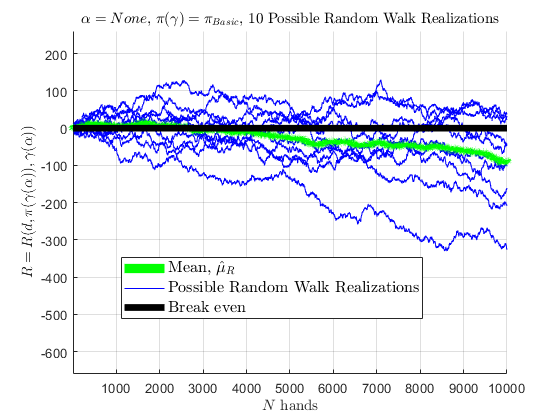
If one were to look at Basic Strategy performance by HiLo count \(\gamma\), for the criteria above:
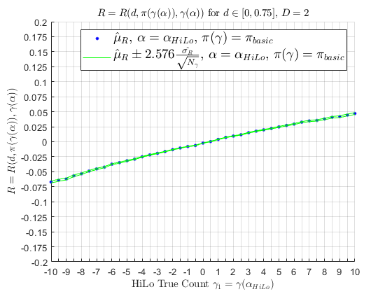
this concave downward behavior, and values, are consistent with Werthamer (2009). If 10 people were to use Basic Strategy for 10,000 hands in a row, represented by 10 simulated random walks, mean of those random walks are seen below; as the number of random walks approach \(\infty\), the mean would converge to \(\hat{\mu}_{R} \approx -0.004\) as the random walks experience the cut-card effect.
Using a training scheme mentioned below, a strategy can be devised such that the strategy is now a function of the true count \(\gamma\), i.e., \(\pi = \pi\left(\gamma\right)\), to increase the player's advantagbe further.
Simulation: Training Algorithm
Various random number generators (RNGs) were explored. Mersenne Twister, and also randomness based on hardware (environmental noise collected from device drivers and other sources when sufficient entropy has been gathered, especially useful as the number of physical nodes of a distributed cluster increase). When billions (or trillions) of simulated Blackjack rounds are performed, one does not want a repeating period of pseudo-random behavior. With proper random number generation, 500 CPU cores of a distributed cluster is used to run a blackjack simulator in C++, validated in previous benchmarks and also run in “human mode” for a human to play and verify bug-free execution of the blackjack engine. A depth \(d=[0,0.75]\) range is used as a cut card in simulations, which is actually faster than shuffling after every first hand of the shoe (which is what most sources do for Basic Strategy development) since the shuffle was slower than a few number of simulated blackjack rounds. However, not just Basic Strategy is being developed, but Basic Strategy deviations based on the count \(\gamma\), so a depth \(d\) is preferred (keeping in mind the cut card effect). An iterative scheme is devised by finding the optimal decision of a (hand type, total, decision) 3-tuplet,\[ \begin{align} \pi_{\text{Optimal}}\left(\gamma_{1}\left(\vec{\alpha}_{\text{HiLo}}\right)\right) = \text{arg}\max\limits_{\pi}R\left(\pi\right), \pi = \{\text{SRh}, \text{SRs},\text{Dh},\text{Ds},\text{H},\text{S},\text{SP},\text{Dsp},\text{SRsp} \} \end{align} \]
When building a basic strategy with a depth range of \([0,d_{\text{max}}]\), and taking the optimal strategy at count 0 (rather than reshuffling after every first draw of the shoe), one must take CCE into account, as it creates a bias in basic strategy results for borderline cases (one observed case is 16vs10). Player totals consisting of many small cards arises more with the possibility of deeper depths of a shoe, resulting in a bias in composition dependent states- because when high cards are already drawn (resulting in less player/dealer Hits, resulting in many cards left, resulting in more rounds to be played until cut card is reached), more small cards remain in the shoe. Example, a player total of 16 (10,6) vs. a dealer upcard of 8 is a state where hilo count is 0, and is a possible first hand from the shoe where the hilo count is 0 before and after hands are dealt. However, only deeper in the shoe can a player total 16 consist of (2,2,2,4,3,3) vs. 8 with a hilo count of 0 after hands dealt, becaue prior to the deal, the hilo count had to be -6, but the hilo count of a new shoe starts at 0. Also, if player total 16 (2,2,2,4,3,3) is drawn, then there are less small cards left to make 16 favorable to Hit, and if there are more rounds of this scenario happening than there are of large cards (due to large cards drawing less due to CCE), a small bias becomes apparentt. One can mitigate for this in the learning algorithms, by mitigating the effect of CCE generally (removing the cut card instead and have a predetermined number of rounds per shoe, or tune the training criteria to avoid abundance of rounds where \(\gamma_{1}\left(\vec{\alpha}_{\text{HiLo}}\right) < 0\) due to CCE bias. The CCE isn't truly ignored, however, as the human player would experience this bias of sampling naturally in real life, as it occurs in the real world.
Notes for this training: when training decisions for specific counts, there are 2 separate places to track the count \(\gamma_{1}\left(\vec{\alpha}_{\text{HiLo}}\right)\) (in rounded intervals of 0.5, only training for \(\gamma_{1}\left(\vec{\alpha}_{\text{HiLo}}\right) \in [-10,10]\)). For betting purposes, the player only knows the \(\gamma_{1}\left(\vec{\alpha}_{\text{HiLo}}\right)\) before hands are dealt, only to be used for betting purposes. For decision purposes, though, the counts used are those before a possible decision can be made, as afterall, training for a \(\pi = \pi\left(\gamma_{1}\left(\vec{\alpha}_{\text{HiLo}}\right)\right)\) is the goal, and the most updated \(\gamma_{1}\left(\vec{\alpha}_{\text{HiLo}}\right)\) up to the point of making a decision is what matters for \(\pi\left(\gamma_{1}\left(\vec{\alpha}_{\text{HiLo}}\right)\right)\). And when trying to learn a hand with a specified type or total, one can't merely force a player to receive the hand total of interest and then randomize the remaining cards; that would affect the likelihood of receiving subsequent hands and add a bias in sampling of hands. One can't force a deck composition at all without introducing a bias, without taking into account the likelihood distribution derived \(\eqref{eq:200}\). One can probably build a function to do so carefully using \(\eqref{eq:200}\), but that wasn't done; here, I would run 1 billion simulations for a chosen {hand type, hand total, action} 3-tuple and whenever the simulations pick up this hand type and hand total being trained (whether it be the initial cards or after a decision is made), the training stores the number of units made/lost for the decision in question for the associated hand type, and hand total.
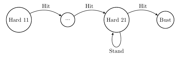
Stage 1 There are 3 types of hands: Hard, Soft, and Pair. If one has a Hard total of 11-21, it will remain Hard, for which Hard 21 is the highest one can reach without busting. Additionally, the Hard total is monotonically increasing if one is to transition by hitting: e.g., a Hard 21 can only bust; a Hard 20 can only turn into a Hard 21 or higher (bust); a Hard 19 can only turn into a Hard 20-21 or higher (bust), and so on. Thus, if one knows the optimal action for Hard 21, then an optimal action for Hard 20 can be reached; if an optimal action for Hard 20 is known, then an optimal action for Hard 19 can be reached, and so on. This logic is used by iterating over all relevant actions (SRh, SRs, Dh, Ds, H, S) from Hard 21 down to Hard 11.
Stage 2 Next, one can realize that a Soft hand (a hand where A can be treated as a 1 or 11), of total \(T_{\text{Soft}}\), upon a transition via a hit, can only turn into a) a Soft hand higher than \(T_{\text{Soft}}\), or b) a Hard total range of \([12, T_{\text{Soft}}]\). Since we already know optimal actions for Hard totals of \([12,T_{\text{Soft}}]\), then optimal actions for Soft hands can be reached.
Stage 3 Next, using optimal actions of Hard \([11-21]\) range and all Soft hands, then a training of Hard \([5,10]\) occurs, since a Hard hand of total \(\le 10\) can turn into any Soft or Hard 12-21. This concludes the training for Hard totals of \([5,10]\).
Stage 4 Lastly, pairs, when split, end up in a Hard or Soft hand (from A,A), and since we have the optimal actions for all non-pair Hard and Soft hands at this point, we can find the optimal decision for pairs after they are split, or not. The difference between pairs and non-pairs, is that when calculating the expected value for pairs, one has to account for the return of all subsequent additional hands resulting from resplitting, to sum up all the gains from splitting. For Hard or Soft, however, only that hand is recorded for expectation calculation (however it is arrived). Also, when the maximum number of splits is reached (typically 3 for any pair, except for A,A where only 1 split is allowed, dependent on the casino's RSA policy), a decision is needed to be made for the pair other than split. In these scenarios, the trained Hard total is used for Hard pairs, except for when the pair is a Soft hand (A,A), for which I force a 'Stay’ action since the casino usually doesn't allow a player to hit in such a scenario, although it is rare altogether (and subject to the modeler's discretion as what to do in such a scenario). Also, for a 2,2 Pair, since there is no defined Hard 4 otherwise, I force a 'Hit’ action. In these scenarios where resplitting limit is reached, I used the resulting Hard (Soft) non-split action on the hand as part of the expectation value of the Pair, not Hard (Soft), which may be subject to perspective of the modeler.
When the training does not know what to do (for example, training in Stage 1, and observes a hard 10), it merely hits (and the hand total 10 is not recorded) to arrive at a Hard hand of interest for Stage 1 to help make the computations more efficient- randomly choosing stay for Hard 10 when in Stage 1 is computationally inefficient. When a pair is reached in Stage 1, it randomly selects to hit or split, just to arrive at a Hard hand of interest (random selection of H or SP is to help reduce bias in composition dependent probabilities and thus, probabilities). This is what makes this training methodology not be perfect: Hard hands (Stages 1, 3) are not trained from the optimal action of Pairs (Stage 4), or optimal action of Softs (stage 2) which may affect the composition dependent probabilities (and thus probabilities) of certain kinds of hands, e.g., 16 (10,6) may be arrived at from 10,10 splitting too often when the action of 10,10 pair is randomly chosen to be SP (and not H) too often.
One way around this, however, could be reinforcement learning such as Q-learning, where the optimal policy of all hand types, totals, is simultaneously arrived gradually (instead of in serial stages). For a hand total, or state, \(s_{t}\), and action, \(a_{t}\), and payout for a hand, \(r_{t}\), the optimal \(a\) for a state can be arrived at with the following converging algorithm:
\[ \begin{align} Q^{\text{new}}\left(s_{t},a_{t}\right)\leftarrow Q\left(s_{t},a_{t}\right) + \alpha\left(r_{t} + \gamma \max\limits_{a} Q\left(s_{t+1},a\right) - Q\left(s_{t},a_{t}\right)\right) \end{align} \]
This reinfinforcement learning is essentially a weighted average of the current value and the new information after an action applied, and a reward is realized. However, this methodology which requires (much) more memory, arrives at similar imperfections when the modeler has to decide how to select the learning rates, \(\alpha\), for such an algorithm. The learning rates, one for each hand total or even transition, could be dynamically updated over time to allow for a learning/exploitation balance, but how to do that remains a similar problem for the serial stages listed above; when the model does not know the optimal policy, how to choose with minimal bias? Regardless of the model, this parameter is subject to proper tuning for better results. The serial metholody arrives at desired results below, for this study.
For every stage, for every hand total, for every action of interest ((SRh, SRs, Dh, Ds, H, S) for Hard/Soft hands, and (SRh, SRs, Dh, Ds, H, S, SRsp, Dsp, SP) for Pair hands), 1 billion simulated hands ran on a cluster of 500 CPU cores, resulting in a confidence interval of every probability in question, and maximal policies were chosen to maximize player return, \(E\left[R\left(d, \pi\left(\gamma\left(\vec{\alpha}_{\text{HiLo}}\right)\right),\gamma_{1}\left(\vec{\alpha}_{\text{HiLo}}\right)| \gamma_{1}\left(\vec{\alpha}_{\text{HiLo}}\right)\right)\right]\), across \(\gamma_{1}\left(\alpha_{\text{HiLo}}\right)\) to arrive at \(\pi\left(\gamma_{1}\left(\alpha_{\text{HiLo}}\right)\right)\).
Simulation: Results; \(\pi_{\text{Optimal}}\left(\gamma_{1}\left(\vec{\alpha}_{\text{HiLo}}\right)\right)\). Card Counting (Hi-Lo)
With counting, the Invariance Theorem no longer applies so the return is a function of true count. For a game with identical conditions as that of the benchmark above,
# of decks: 2
Dealer hits on soft 17 (H17)
Player may resplit to four hands, except aces (where 1 split only is allowed) (no RSA)
No drawing to split aces beyond 1 card
Double on any 2 cards, no restrictions (DOA)
Double after split allowed (DAS)
Blackjack payout: 3:2
Deck depth: [0,0.75]
Flat betting (betting 1 unit always)
Insurance payout: 2:1
Double on any pair
Late Surrender allowed
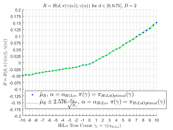
we perform a strategy training for \(\pi_{\text{Optimal}}\left(\gamma_{1}\left(\vec{\alpha}_{\text{HiLo}}\right)\right)\) and we see the following Basic Strategy deviations using HiLo count. Notable Basic Strategy deviations from this model training include: hitting on Hard 12 (instead of staying) v 4 when \(\gamma_{1}\left(\vec{\alpha}_{\text{HiLo}}\right) < 0\), splitting 10,10 (instead of staying) vs 6 when \(\gamma_{1}\left(\vec{\alpha}_{\text{HiLo}}\right) > 3\), hitting A,A (instead of splitting) vs. A when \(\gamma_{1}\left(\vec{\alpha}_{\text{HiLo}}\right) \le -7.5 \), doubling on Soft 20 (instead of staying) vs. 6 when \(\gamma_{1}\left(\vec{\alpha}_{\text{HiLo}}\right) \ge 5\), surrendering on Hard 15 (instead of hitting) vs. 9 when \(\gamma_{1}\left(\vec{\alpha}_{\text{HiLo}}\right) \ge 2.5\), and much more. I will call this HiLo Optimal Strategy, \(\pi_{\text{Optimal}}\left(\gamma_{1}\left(\vec{\alpha}_{\text{HiLo}}\right)\right)\) rather than Basic Strategy, \(\pi_{Basic}\).
As for insurance, there is ambiguity in what the actual index is for \(\alpha_{\text{HiLo}}\); Werthamer claims that it is depth dependent, and instead of 3, it may actually be closer to 4 for greater depths (Werthamer, 2009). To avoid a depth dependent optimal Insurance decision, a perfect insurance count is devised. The Perfect Insurance count is a counting system to determine when to insure your hand or not; to derive it, we start with the Insurance payout of 2:1, and the scenario this action is to take place is when the dealer has an Ace upcard. The sample space of probabilities for dealer having blackjack is reduced when there is a 10 (\(j=10\)) value hole card for the dealer. To ensure positive expectation, with an initial bet size of \(1\) unit, Insurance bet of \(\frac{1}{2}\) unit,
\[ \begin{align*} E[\text{Insurance}] > 0 \implies (-0.5)P\left(\text{not a 10 hole card}\right) + (2)P\left(\text{10 hole card}\right) > 0 \end{align*} \]
\[ \begin{align*} \implies (-0.5)\frac{\tilde{M} - \tilde{m}_{10}}{\tilde{M}} + (2)\frac{\tilde{m}_{10}}{\tilde{M}} > 0 \\ \implies (-0.5)\frac{ - \tilde{m}_{10}}{\tilde{M}} + (2)\frac{\tilde{m}_{10}}{\tilde{M}} > 0.5 \\ \implies (1.5)\frac{\tilde{m}_{10}}{\tilde{M}} > 0.5 \\ \implies \frac{\tilde{m}_{10}}{\tilde{M}} > \frac{1}{3} \\ \implies \frac{\nu_{10} - m_{10}}{52D - M} > \frac{1}{3} \\ \implies \frac{\nu_{10} - m_{10}}{52D - (m_{10} + m_{j\ne 10})} > \frac{1}{3} \\ \implies \frac{52Dl_{10}^{0} - m_{10}}{52D - (m_{10} + m_{j\ne 10})} > \frac{1}{3} \\ \implies 3\left(52Dl_{10}^{0} - m_{10}\right) > 52D - m_{10} - m_{j\ne 10} \\ \implies 3\left(16D - m_{10}\right) > 52D - m_{10} - m_{j\ne 10} \\ \implies 48D - 3 m_{10} > 52D - m_{10} - m_{j\ne 10} \\ \implies m_{j\ne 10} - 2 m_{10} > 4D \end{align*} \]
So we have arrived at the Perfect Insurance running count: when \(\tilde{m}\cdot\alpha_{\text{Perfect Insurance}} > 4D\), insure; else, don't insure. In addition to HiLo, the multi-parameter counting system used for analyzing performance is used:
| A | 2 | 3 | 4 | 5 | 6 | 7 | 8 | 9 | 10 | |
| \(j\) | 1 | 2 | 3 | 4 | 5 | 6 | 7 | 8 | 9 | 10 |
| \(\lambda=1\) | \(\alpha_{1,1}\) | \(\alpha_{1,2}\) | \(\alpha_{1,3}\) | \(\alpha_{1,4}\) | \(\alpha_{1,5}\) | \(\alpha_{1,6}\) | \(\alpha_{1,7}\) | \(\alpha_{1,8}\) | \(\alpha_{1,9}\) | \(\alpha_{1,10}\) |
| HiLo, \(\vec{\alpha}_{1}\) | -1 | 1 | 1 | 1 | 1 | 1 | 0 | 0 | 0 | -1 |
| \(\lambda=\Lambda=2\) | \(\alpha_{2,1}\) | \(\alpha_{2,2}\) | \(\alpha_{2,3}\) | \(\alpha_{2,4}\) | \(\alpha_{2,5}\) | \(\alpha_{2,6}\) | \(\alpha_{2,7}\) | \(\alpha_{2,8}\) | \(\alpha_{2,9}\) | \(\alpha_{2,10}\) |
| Perfect Insurance, \(\vec{\alpha}_{2}\) | 1 | 1 | 1 | 1 | 1 | 1 | 1 | 1 | 1 | -2 |
Using \(\vec{\alpha}_{1}=\vec{\alpha}_{\text{HiLo}}\) for \(\pi_{\text{Optimal}}\left(\gamma_{1}\left(\vec{\alpha}_{\text{HiLo}}\right)\right)\), \(B\left(\gamma_{1}\left(\vec{\alpha}_{\text{HiLo}}\right)\right)=1\) \(\forall\) \(\gamma_{1}\left(\vec{\alpha}_{\text{HiLo}}\right)\), and \(\vec{\alpha}_{2}=\vec{\alpha}_{\text{Perfect Insurance}}\) for insurance decisions \(I\left(\gamma_{2}\left(\vec\alpha_{\text{Perfect Insurance}}\right)\right)\) only, for 1 billion simulations,
\[ \hat{R}_{\text{Shoe}}\left(\vec{\alpha}_{1},\vec{\alpha}_{2}\right) = \frac{1}{d_{\text{max}}}\int_{0}^{d_{\text{max}}}dd \int d\gamma_{1}\left(\vec{\alpha}_{\text{HiLo}}\right) \rho\left(\gamma_{1}\left(\vec{\alpha}_{\text{HiLo}}\right)\right)E\left[R\left(d,\pi_{\text{Optimal}}\left(\gamma_{1}\left(\vec{\alpha}_{1}\right)\right),I\left(\gamma_{2}\left(\vec{\alpha}_{2}\right)\right)\right) | \vec{\gamma}\right] \approx -0.001. \]
\(\hat{R}_{\text{Shoe}}\left(\vec{\alpha}_{1},\vec{\alpha}_{2}\right)\), for flat betting is still slightly negative but still more positive than \(\hat{R}_{\text{Basic Strategy}} \approx -0.004\) (all including cut card effect). If \(B\left(\gamma_{1}\left(\vec{\alpha}_{\text{HiLo}}\right)\right) = 2\) for \(\gamma_{1}\left(\vec{\alpha}_{\text{HiLo}}\right) \ge 1\) and \(B\left(\gamma_{1}\left(\vec{\alpha}_{\text{HiLo}}\right)\right) = 1\) otherwise, for 1 billion simulations,
\[ \begin{equation} \hat{R}_{\text{Shoe}}\left(\vec{\alpha}_{1},\vec{\alpha}_{2}\right) = \frac{1}{d_{\text{max}}}\int_{0}^{d_{\text{max}}}dd \int d\gamma_{1}\left(\vec{\alpha}_{\text{HiLo}}\right) \rho\left(\gamma_{1}\left(\vec{\alpha}_{\text{HiLo}}\right)\right)B\left(\gamma_{1}\left(\vec{\alpha}_{\text{HiLo}}\right)\right)E\left[R\left(d,\pi_{\text{Optimal}}\left(\gamma_{1}\left(\vec{\alpha}_{1}\right)\right),I\left(\gamma_{2}\left(\vec{\alpha}_{2}\right)\right)\right) | \vec{\gamma}\right] \approx +0.0075. \; \llap{\mathrel{\boxed{\phantom{ \hat{R}_{\text{Shoe}}\left(\vec{\alpha}_{1},\vec{\alpha}_{2}\right) = \frac{1}{d_{\text{max}}}\int_{0}^{d_{\text{max}}}dd \int d\gamma_{1}\left(\vec{\alpha}_{\text{HiLo}}\right) \rho\left(\gamma_{1}\left(\vec{\alpha}_{\text{HiLo}}\right)\right)B\left(\gamma_{1}\left(\vec{\alpha}_{\text{HiLo}}\right)\right)E\left[R\left(d,\pi_{\text{Optimal}}\left(\gamma_{1}\left(\vec{\alpha}_{1}\right)\right),I\left(\gamma_{2}\left(\vec{\alpha}_{2}\right)\right)\right) | \vec{\gamma}\right] \approx +0.0075…. }}}} \end{equation} \]
An overall player edge of \(\approx +0.0075\) \(\left(+0.75\%\right)\) is reached (99% confidence interval for 1 billion hands: [0.00739 0.00765]). \(\pi\left(\gamma_{1}\left(\alpha_{\text{HiLo}}\right)\right)\) reduces the dependence on a large betting spread, and reduces variance of bankroll over time, which is different typically how HiLo is used (not many sources emphasize the use of \(\pi\left(\gamma_{1}\left(\alpha_{\text{HiLo}}\right)\right)\).
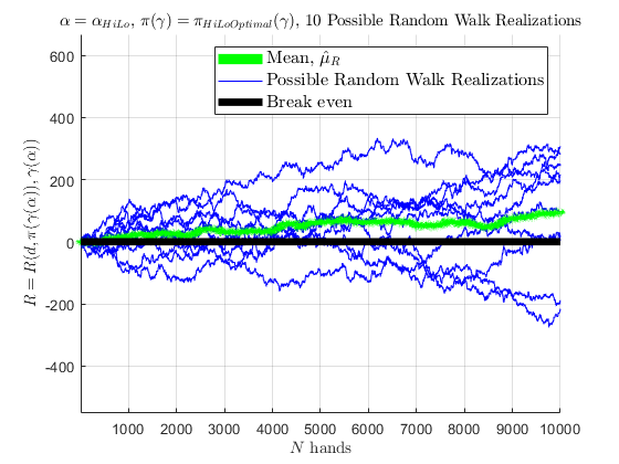
If 10 people were to use \(\pi_{\text{Optimal}}\left(\gamma\left(\alpha_{\text{HiLo}}\right)\right)\) for 10,000 hands in a row, represented by 10 simulated random walks, a mean of those random walks are seen below; as the number of random walks approach \(\infty\), the mean would converge to \(\hat{\mu}_{R} \approx +0.0075\) as the random walks experience the cut-card effect.
Simulation: Near Optimal Play
The above section is using just 2 counting vectors; \(\vec{\alpha}_{\text{HiLo}}\) for strategy, betting, and \(\vec{\alpha}_{\text{Perfect Insurance}}\) for insurance only, and a betting scheme where \(B\left(\gamma_{1}\left(\vec{\alpha}_{\text{HiLo}}\right)\right)=2\) for \(\gamma_{1}\left(\vec{\alpha}_{\text{HiLo}}\right)\ge 1\), and \(B\left(\gamma_{1}\left(\vec{\alpha}_{\text{HiLo}}\right)\right)=1\) for \(\gamma_{1}\left(\vec{\alpha}_{\text{HiLo}}\right) < 1\). To calculate the optimal counting vector \(\left(\vec{\alpha}^{\text{Optimal}}_{1},…,\vec{\alpha}^{\text{Optimal}}_{\Lambda}\right)\), \(\Lambda > 2\), that would result in an optimal return \(E\left[R_{\text{Shoe}}\right]\) higher than \(E\left[R\left(d, \pi\left(\gamma\left(\alpha_{\text{HiLo}},\pi_{\text{Optimal}}\left(\alpha_{\text{HiLo}}\right)\right)\right)\right)\right]\), for \(B\left(\vec{\gamma}\right)=1\) \(\forall\) \(\vec{\gamma}\),the following optimization is to be performed:\[ \begin{equation} \left(\vec{\alpha}^{\text{Optimal}}_{1},…,\vec{\alpha}^{\text{Optimal}}_{\Lambda}\right) =\underset{\vec{\alpha}_{1}, …, \vec{\alpha}_{\Lambda}}{\text{argmax }} \frac{1}{d_{\text{max}}}\int_{0}^{d_{\text{max}}}dd \int d\vec{\gamma} \rho\left(\vec{\gamma}\right)E\left[R\left(d,\pi_{\text{Optimal}}\left(\gamma_{1}\left(\vec{\alpha}_{1}\right),…\gamma_{\Lambda}\left(\vec{\alpha}_{\Lambda}\right)\right)\right) | \vec{\gamma}\right]. \; \llap{\mathrel{\boxed{\phantom{…..\left(\vec{\alpha}^{\text{Optimal}}_{1},…,\vec{\alpha}^{\text{Optimal}}_{\Lambda}\right) =\underset{\vec{\alpha}_{1}, …, \vec{\alpha}_{\Lambda}}{\text{argmax }} = \frac{1}{d_{\text{max}}}\int_{0}^{d_{\text{max}}}dd \int d\vec{\gamma} \rho\left(\vec{\gamma}\right)E\left[R\left(d,\pi_{\text{Optimal}}\left(\gamma_{1}\left(\vec{\alpha}_{1}\right),…\gamma_{\Lambda}\left(\vec{\alpha}_{\Lambda}\right)\right)\right) | \vec{\gamma}\right].}}}} \end{equation} \]
Using a numerical solver like SP-GOPT, this can be done, however it becomes cumbersome as a single evaluation of the objective function can take hours long, and \(\left(\vec{\alpha}^{\text{Optimal}}_{1},…,\vec{\alpha}^{\text{Optimal}}_{\Lambda}\right)\) can be very computationally expensive. However, tricks can be performed for computational efficiency and knowledge of scenarios can reduce the search space as well as the objective function evaluation time. Werthamer approaches this analytically, however, for \(\Lambda>2\), the machinery becomes very cumbersome and was not pursued in his book. As far as I know, a multi-parameter solution for \(\left(\vec{\alpha}^{\text{Optimal}}_{1},…,\vec{\alpha}^{\text{Optimal}}_{\Lambda}\right)\) for \(\Lambda>2\) is not published anywhere.
Final Note
I hope my family and friends believe me now when I say I am not addicted to gambling; rather, I'm a taker of calculated risk and reward…References
1. Preston, P., 2017, “Edward Thorp's 20% Annual Return for 30 Years,” Forbes, March 13, https://www.forbes.com/sites/prestonpysh/2017/03/13/edward-thorp-blackjack-beat-the-dealer/?sh=29e3db6713de
2. Kurson, K. “Thorp's market activities”. Webhome.idirect.com. Archived from the original on February, 2003. https://web.archive.org/web/20051031090504/http://webhome.idirect.com/ blakjack/edthorp.htm
3. Shackleford, M., 2019, “Blackjack expected Returns for six decks and dealer hits on soft 17.” The Wizard of Odds. https://wizardofodds.com/games/blackjack/appendix/9/6dh17r4
4. Werthamer, N. R., “Risk and Reward: The Science of Casino Blackjack”. 2009.
2. Wikipedia contributors. (2022, October 21). “Blackjack.” Wikipedia. https://en.wikipedia.org/wiki/Blackjack
5. Depaulis, Thierry (April–June 2010). “Dawson's Game: Blackjack and the Klondike”. In Peter Endebrock (ed.). The Playing-Card. Journal of the International Playing-Card Society. Vol. 38 (4). The International Playing-Card Society. ISSN 0305-2133.
6. Baldwin, Rober, Wilbert E. C., Herbert M., James P. M., “The Optimum Strategy in Blackjack”, Journal of the American Statistical Association, 51, 429-439 (1956).
7. Snyder, Arnold, “Blackbelt in Blackjack”, Cardoza Publishing, Las Vegas, NV, 3rd edition (2005); “The Big Book of Blackjack”, Cardoza Publishing, Las Vegas, NV (2006)
8. Griffin, P. A., “The Theory of Blackjack”, Huntington Press, Las Vegas, NV, 6th edition (1999).
9. Wikipedia contributors. (2022, September 30). “Don Johnson (gambler)”. https://en.wikipedia.org/wiki/Don_Johnson_(gambler)
10. Wikipedia contributors. (2019, March 30). James Grosjean. Wikipedia. https://en.wikipedia.org/wiki/James_Grosjean
11. Thorp, E. O., “Does Basic Strategy Have the Same Expectation for Each Round?”, in Vancura, O., J.A. Cornelius, and W.R. Eadington (eds.), “Finding the Edge: Mathematical Analysis of Casino Games”, University of Nevada, Reno (2000). http://www.edwardothorp.com/wp-content/uploads/2016/11/DoesBasicStrategyHaveTheSameExpectionForEachRound.pdf
12. Shackleford, M., 2015, “Blackjack House Edge Calculator”. https://wizardofodds.com/games/blackjack/calculator